LS-DYNA: Difference between revisions
| Line 403: | Line 403: | ||
Decomposition is often ignored by LS-DYNA users. However, it allows for a huge savings of computational time for many simulations. Let’s take a look at the problem of soil penetration, with a quarter of the model shown below. In the simulation a rigid pad is pressed down into the soil with the rate of 1 in/sec. The first two inches of penetration are simulated. The Z-axis is pointing upward and the (0,0,0) point is at the top layer of the soil (brown in the figure). | Decomposition is often ignored by LS-DYNA users. However, it allows for a huge savings of computational time for many simulations. Let’s take a look at the problem of soil penetration, with a quarter of the model shown below. In the simulation a rigid pad is pressed down into the soil with the rate of 1 in/sec. The first two inches of penetration are simulated. The Z-axis is pointing upward and the (0,0,0) point is at the top layer of the soil (brown in the figure). | ||
[[Image:Soil_model.jpg|thumb|none|left|200px|alt=Soil penetration model|Soil penetration model]] | [[Image:200px-Soil_model.jpg|thumb|none|left|200px|alt=Soil penetration model|Soil penetration model]] | ||
Now consider three different decomposition methods for eight cores, as defined in the pfile: | Now consider three different decomposition methods for eight cores, as defined in the pfile: | ||
| Line 432: | Line 432: | ||
This gives the three decompositions shown in the figure below: | This gives the three decompositions shown in the figure below: | ||
[[Image:Decomp_soil.jpg|thumb|none|left|400px|alt=Decomposition methods (from left) default, wedge type, cylindrical|Decomposition methods (from left) default, wedge type, cylindrical]] | [[Image:400px-Decomp_soil.jpg|thumb|none|left|400px|alt=Decomposition methods (from left) default, wedge type, cylindrical|Decomposition methods (from left) default, wedge type, cylindrical]] | ||
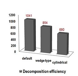
The run time for these jobs is shown in the graph. The third decomposition type was most efficient and allowed for a saving of ~34.7% of the computation time. The second decomposition method gave a saving of ~18.0%. | The run time for these jobs is shown in the graph. The third decomposition type was most efficient and allowed for a saving of ~34.7% of the computation time. The second decomposition method gave a saving of ~18.0%. | ||
[[Image:Decomp_efficiency.jpg|thumb|none|left|250px|alt=Decomposition efficiency|Decomposition efficiency]] | [[Image:250px-Decomp_efficiency.jpg|thumb|none|left|250px|alt=Decomposition efficiency|Decomposition efficiency]] | ||
See Appendix O of the LS-DYNA Keyword User’s Manual, Version 971 for an explanation the use of pfiles. | See Appendix O of the LS-DYNA Keyword User’s Manual, Version 971 for an explanation the use of pfiles. | ||
Revision as of 16:53, February 3, 2021
Terminology
In our documentation,
- LS-DYNA refers to both SMP-DYNA and MPP-DYNA
- SMP-DYNA refers to the single node, shared-memory version of LS-DYNA
- MPP-DYNA refers to the MPI verion of LS-DYNA
Getting started
modules
You'll need to load the base LS-DYNA module to use MPP-DYNA on the cluster. In most cases this is the only module you'll need to load.
We also have version-specific modules for each version of MPP-DYNA. Each of these modules adds the single and double precision versions of MPP-DYNA to your PATH as "mpp_s" and "mpp_d", respectively, along with and "l2a_s" and "l2a_d", the single and double precision versions of l2a. Each module also sets up your environment for the latest installed version of the appropriate MPI library. You will not need to load these modules at the command line unless you intend to run one of these programs manually, as LS-DYNA#qsub-mpp-dyna will load the appropriate module for you automatically.
The version-specific MPP-DYNA modules are named ls-dyna/mpp/<compiler>-<MPI library>/<version>. SMP-DYNA modules are named ls-dyna/smp/<version>. For example:
ls-dyna/mpp/intel-hp/r4.2.1
ls-dyna/smp/7600.2.1224
You can see a list of all available modules with the command
module -t avail ls-dyna
Which version should I use?
In our testing with the 3cars, car2car, and neon_refined_revised models from TopCrunch, we've found that the fastest binaries are generally the "pgi-hp" versions, and that the 7600.12.1224 version is the fastest of those. However, newer versions have numerous bugfixes and enhancements. We do not currently recommend the hybrid versions, as they're considerably slower than the pure MPP versions. Versions with "alpha" or "beta" in the name may or may not work.
If you'd like us to install a version we don't have, please contact us.
qsub-mpp-dyna on Phoenix
Please see below for running LS-Dyna on Zephyr. The qsub-mpp-dyna tool on Zephyr has been replaced with qsub-dynatui.py.
The qsub wrapper script "qsub-mpp-dyna" simplifies the submission of MPP-DYNA jobs to Torque. The script will automatically write and submit a Torque job script for you. It will also ensure that the job releases its licenses back to the license server.
Usage: qsub-mpp-dyna
       [ --cores <cores> ]
       [ --decomp ]
       [ [--dyna] <mpp-dyna arguments> ]
       [ --hours <hours> | --minutes <minutes> ]
       [ --lsopt <command-file> ]
       [ --nosubmit ]
       [ --single | --double ]
       [ --32 ]
       [ --64 ]
       [ < qsub arguments> ]
       --module <ls-dyna module> | --smp <smp-version>

Defaults: --double
          --32
          -j oe -A dyna

Examples:
       qsub-mpp-dyna --cores 32 i=crash.k p=pfile --hours 1 --module pgi-hp/r4.2.1
qsub-mpp-dyna --cores 128 --dyna i=crash.k p=pfile --minutes 90 --module pgi-hp/r4.2.1 --single -N neon
       qsub-mpp-dyna --module pgi-hp/7600.2.1224 i=crash.k -l nodes=16:ppn=4,walltime=24:00:00
       qsub-mpp-dyna -l nodes=16:ppn=8,walltime=24:00:00 i=crash.k r=d3dump01 --module intel-hp/r4.2.1-sharelib
       qsub-mpp-dyna --lsopt crash.opt i=barrier.k --smp r4.2.1 --hours 72 --cores 4 --nosubmit
       qsub-mpp-dyna -l nodes=8:ppn=8,walltime=24:00:00 i=crash.k r=d3dump01 --module pgi-hp/r4.2.1
If the --nosubmit option is used, a PBS job script will be written but not submitted. The job will then need to be submitted manually with qsub.
Note that
- qsub-mpp-dyna by default will use 32 bit IEEE format for d3plot and d3thdt files. To use 64 bit format, use the --64 command line switch.
- if your pfile contains the following line as part of the "dir" specification (see Appendix O of the LS-DYNA Keyword User’s Manual, Version 971)
global GLOBAL local LOCAL
then the job file will dynamically replace this with
global $PBS_JOBID local /scratch/$PBS_JOBID
where /scratch/$PBS_JOBID is local to each node running the job.
qsub-dynatui.py on Zephyr
First, load the lstc/base module:
$ module load lstc/base
To obtain a list of options and parameters for qsub-dynatui.py:
$ qsub-dynatui.py --help
usage: qsub-dynatui.py [-h] [-v] -i InputFile [-j JobName] [-M Email]
                      [-d Days] [-r Hours] [-m Minutes] -c Cores -l Module
                      [-o LSOpt] -p Precision [-s Submit] [-y DynaArgs]
                      [-q QsubArgs]
LS-Dyna Job Submission Tool
optional arguments:
 -h, --help    show this help message and exit
 -v            show program's version number and exit
 -i InputFile  (Enter input file, i.e. 3cars_shell2_150ms.k)
 -j JobName    (Enter job name, i.e. 3Cars_Run1
 -M Email      (Enter E-Mail for notification, i.e. [email protected])
 -c Cores      (Number of cores, i.e. 16)
 -l Module     (Choose module, i.e. 3 for lstc/intel/r5.0)
 -o LSOpt      (Enter 'y' if using LS-Opt. Default no)
 -p Precision  (Choose precision, i.e. [s]ingle or [d]ouble)
 -s Submit     (Enter 'n' to create pbs script. Default yes)
 -y DynaArgs   (LS-Dyna args, i.e. -y "memory1=200m memory2=100m", etc...)
 -q QsubArgs   (Enter queue, i.e. 64gb and 128gb. Default is 32gb)
WALLTIME:
 -d Days       (Number of days job should run, i.e. 1)
 -r Hours      (Number of hours job should run, i.e. 12)
 -m Minutes    (Number of minutes job should run, i.e. 30)
Valid LS-Dyna Modules are:
       0:  lstc/OpenMPI/r5.1.1_65550
       1:  lstc/OpenMPI/r6.1.1_81075_BETA
       2:  lstc/OpenMPI/r4.2.1
       3:  lstc/OpenMPI/r6.0.0_71488
       4:  lstc/OpenMPI/r6.1.0_74904
       5:  lstc/OpenMPI/r5.0
       6:  lstc/intel/r4.2.1
       7:  lstc/intel/r7_0_0_79069
       8:  lstc/intel/r6.0.0_71488
       9:  lstc/intel/r6.1.0_74904
       10:  lstc/intel/r6.1.1_79036
       11:  lstc/intel/r5.0
       12:  lstc/hyb/OpenMPI/r6.1.0_74904
       13:  lstc/hyb/intel/r6.1.0_74904
       14:  lstc/smp/r7.0.0
       15:  lstc/smp/r5.0
       16:  lstc/smp/r6.1.0
For example, suppose the following job needs to be created:
- Number of cores desired: 32
- Number of hours the job is expected to run: 60
- Main input file: main.k
- LS-Dyna arguments: memory=950m, memory2=100m p=pfile
- LS-Dyna module to use: Intel release r6.1.0_74904
- Precision: Single
The following command can be issued to satisfy the requirements above:
$ qsub-dynatui.py -c 32 -r 60 -i main.k -l 5 -p s -y "memory=950m memory2=100m p=pfile"
Breakdown of paramenters passed:
- -c 32, represents 32 cores.
- -r 60, from WALLTIME represents 60 hours. One can also specify days and hours by using the '-d' flag.
- -i main.k, the main LS-Dyna input file is main.k
- -l 5, this is the lowercase letter 'L'. The number 5 represents the 5th module from 'Valid LS-Dyna Modules'. In this particular case it is 'lstc/intel/r6.1.0_74904'. Specifying module number 6 would yield in 'lstc/intel/r5.0', and so forth.
- -p s, is single precision.
- -y "memory=950m memory2=100m p=pfile", All LS-Dyna parameters must be specified using the '-y' flag and enclosed in double quotes as shown in the example.
By default, jobs are submitted automatically unless the submit flag (-s) is set to 'n' for no submit.
Specifying memory requirements
In SMP-DYNA, the amount of memory allocated for the problem can be specified on the command line using the memory keyword:
memory=XXXm
or in the k-file by using
*KEYWORD MEMORY=XXXm
where XXX is the number of mega words (4 bytes for single-precision, 8 bytes for double-precision) of memory to be allocated. For MPP-DYNA you would use the keywords memory1 and memory2:
memory1=YYYm memory2=ZZZm
MPP-DYNA will assign the amount of memory1 to the core performing the decomposition of your job, whereas memory2 will be assigned for the remaining cores.
For example, specifying
memory=270m
for double precision MPP-DYNA would result in the allocation of 270 mega words, or 2.16 GB (= 270 M * 8 B) of memory for each core. Most of our compute nodes have 1 GB per core, which means this job won't run. If you specify
memory1=270m memory2=70m
the total requested memory for the node will be 270 mega words + 3 * 70 mega words = 480 mega words, or 3.84 GB (= (270 M + 3*70 M) * 8 B). The value of memory2 drops nearly linearly with the number of cores used to run the program. (See Appendix O: LS-DYNA MPP User Guide of the LS-DYNA Keyword User's Manual for more info.)
Using smp version of LS-DYNA
To use smp version of LS-DYNA on the cluster you need to choose one of the "smp" modules. Switches "--modules" and "--smp" are mutually exclusive. In order to submit your smp job to more than one core you need to specify also number of CPU's in the input file as foolows:
*KEYWORD NCPU=N
where N is ranging from 1 to 8 for our system.
Decomposing and solving separately
If the memory on a standard compute node (8 GB) is not enough to perform decomposition of your MPP-DYNA job, you can run the job in two stages. The decomposition can be run on a node with 32 GB of memory, with the rest of the calculations performed on standard compute nodes.
For example, to decompose on a single 32 GB node you could use one of the following commands:
qsub-mpp-dyna -q thirtytwogb i=<your-dyna-input> p=pfile_dec --cores 1 memory1=1000m memory2=100m --module pgi-hp/r4.2.1 --hours 1 -N decomp
and then to compute on 4 standard nodes when the decomposition is finished,
qsub-mpp-dyna -W depend=afterany:<decomp-job-id> --cores 32 --hours 24 i=<your-dyna-input> p=pfile_exe -N <job-name>
(The dependency shouldn't be specified if the decomposition job has already completed.)
The pfile (in this example pfile_dec) controls whether decomposition is performed. The essential part is:
decomposition {
    numproc <number-of-cores-that-will-run-your-job>
    file decomp_data
}
This file will cause the job to be divided into the number of cores you specify; after the decomposition, no further calculations will be performed (assuming the number of cores is > 1). In this case, the decomposition data will be written to the file "decomp_data.pre" (for versions before R4) or "decomp_data.lsda" (for versions R4 and later). Note that the "file" keyword is required, although the manual says it isn't.
The pfile for running already decomposed job (in this example pfile_exe) will only contain the name of the file with the decomposition data:
decomposition {
    file decomp_data
}
See Appendix O of the LS-DYNA Keyword User’s Manual, Version 971, for other decomposition options.
Viewing the decomposition
If you want to view the decomposition within LS-PREPOST use keyword "show" in your pfile. Note that only one d3plot file will be created and no further calculations will be performed.
decomposition {
    numproc <number-of-cores-that-will-run-your-job>
    show
}
User subroutines
User subroutines in MPP LS-DYNA
To use your own subroutines with MPP-DYNA, first load a "sharelib" module. For example,
module load ls-dyna/intel-hp/r4.2.1-sharelib
Then make a copy of LSTC's source files, and change to that directory. (Change usermat_d to usermat_s if you're using single-precision.)
cp -a $MPP_DYNA_ROOT/usermat_d .
cd usermat_d
After making your changes to the files in usermat_d, run
make
This will create the file libmpp971_d_53323.53442_usermat.so, which is a library needed by mpp_d and mpp_s. You will need to tell MPP-DYNA where to find this file. You do this with the environment variable LD_LIBRARY_PATH.
For example, say that after creating the library, you cd to your previous directory, then move the library to that directory:
cd ..
mv usermat_d/libmpp971_d_53323.53442_usermat.so .
You would then submit your job like this:
qsub-mpp-dyna --module intel-hp/r4.2.1-sharelib -v LD_LIBRARY_PATH=`pwd` ...
However, you can put the library file anywhere you like, as long as you set LD_LIBRARY_PATH to the directory containing the library. If you put it in ~/lib, you would submit the job with
qsub-mpp-dyna --module intel-hp/r4.2.1-sharelib -v LD_LIBRARY_PATH=~/lib ...
Note that user subroutines are supported for the combination of Intel compiler and HP-MPI only.
User subroutines in SMP LS-DYNA
To use your own subroutines with SMP LS-DYNA, first load one of smp_u modules by command:
module load ls-dyna/smp_u/r4.2.1
or
module load ls-dyna/smp_u/r5.0
Then make a copy of LSTC's source files from:
/mnt/gpfs/soft/lstc/ls-dyna/ls971/R5.0-umat/intel64
if you loaded the r5.0 module, or from
/mnt/gpfs/soft/lstc/ls-dyna/ls971/R4.2.1-umat/xeon64
if you loaded the r4.2.1 module. While in your work directory, use the command:
cp -a /mnt/gpfs/soft/lstc/ls-dyna/ls971/R5.0-umat/intel64/ umat
Change to the umat directory where the files were copied:
cd umat
Now make modifications in the dyn21.f file to the user subroutine(s) you want to change. After this step is finished run the make command:
make
After a while the ls971 file will be created. Move it to the work directory where you have your LS-DYNA input file (k file). For example:
cd ..
mv umat/ls971 .
Here is an example of command to submit your job with smp user defined executable using qsub-mpp-dyna-umat script:
qsub-mpp-dyna-umat --smp_u r5.0 --cores 8 i=my_input_file.k --hours 24 memory1=200m memory2=85m -N my_job_name
Note 1: the qsub-mpp-dyna-umat has the same usage as the qsub-mpp-dyna script.
Note 2: only double precision objects for creating ls971 are available on the cluster. If you need single precision objects or other version of LS-DYNA please contact us via e-mail.
Licenses
Our license allows for 500 concurrent LS-DYNA and MPP-DYNA processes.
If you don't use qsub-mpp-dyna, please submit your jobs to the dyna account:
qsub -A dyna ...
qsub-mpp-dyna does this automatically.
Note that the LSTC license server does not accurately keep track of the number of licenses in use on quad-core CPUs for some older versions of MPP-DYNA. Consequently, lstc_qrun and qdyna may report the wrong number of licenses in use.
lstc_license_count reports the correct license usage. If lstc_license_count says there are no licenses available, your job will not run immediately, regardless of what lstc_qrun and qdyna say.
License manager commands
lstc_license_count
Shows how many DYNA licenses are free.
lstc_qrun
Shows what DYNA jobs are using DYNA licenses. The output will be something like
    User             Host          Program              Started       # procs
-----------------------------------------------------------------------------
ac.berna    [email protected]. LS-DYNA_971      Fri Jul 10 08:15     4
User names will be truncated to 8 characters. The format of the "Host" field is "<PID>@<lowest-numbered-node>-ge.default". ("PID" is "process ID"; this is different from the PBS job ID.)
qdyna
Shows how many DYNA licenses are currently used per user.
lstc_qkill <job>
Forces the LSTC license server to release licenses for <job>, where <job> is the "Host" field in the output of lstc_qrun.
lstc_license_cleanup
Kills stray MPP-DYNA processes, and frees their licenses. This needs to be run in the directory where the PBS job was submitted. To remove licenses for all your jobs, run this command:
lstc_qrun | grep `whoami` | awk '{print $2}' | while read job; do lstc_qkill $job; done
Submitting jobs in graphical mode
Creating job scripts, submitting jobs and checking their status can be performed also in graphical mode. Once you log into the cluster using NoMachine or other software you can run qsub-dyna-gui application (with qsub-dyna-gui command). To create a new job script using qsub-dyna-gui you will have to go through the tabs from the left to the right side and input at least required data: input file, LS-DYNA version and number of nodes. Other fields are optional only and for some of them default values will be assigned if not entered by the user. For detailed information please go to QSUB-DYNA-GUI.
Notes
Single- vs. double-precision
Models that run fine with PC-DYNA using single-precision may fail with divide-by-zero errors on the cluster unless double-precision is used. This seems to be due to differences in how PC-DYNA and MPP-DYNA do floating-point arithmetic. Double-precision jobs are likely to run about 20% slower than single-precision jobs, however.
Submitting multiple jobs
There can be a delay of several seconds from the time MPP-DYNA is invoked to the time it contacts the license server to obtain licenses. This can result in the license server not having enough licenses to run a job, even though there were enough available when the job was submitted. To avoid this problem, it's best to allow at least 10 seconds between job submissions.
Hung jobs
If your job isn't making any progress (for example, not writing to any files), it's likely that MPP-DYNA is in an infinite loop. You can use lstc_qrun to see if the job is still in contact with the license server. If not, please delete it from the PBS queue using qdel.
Dumping restart files
If you belatedly realize that the requested wall time for your job is insufficient to reach the termination time specified in the k-file, you can have LS-DYNA write restart files by creating a D3KIL file containing the appropriate switch control. For example:
echo sw3 > D3KIL
will create a D3KIL file containing the "sw3" switch, causing LS-DYNA to write restart files and continue the run. "sw1" will result in writing restart files and then termination of the job. LS-DYNA periodically looks for D3KIL file and if found, the sense switch will be invoked and the D3KIL file deleted. You can then run a restart job by submitting your job with the same command as previously, adding to the command line only
r=d3dump01
For long jobs we recommend that you generate restart files ("sw3") once a day, to make it easier to recover from the failure of a node on which your job is running.
The "Getting Started" section of the Keyword manual has more info about the use of sense switches.
More nodes doesn't always mean faster
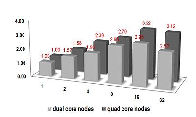
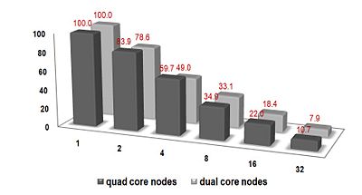
Requesting more nodes for your job doesn't always mean that you will get your results faster. As the number of cores increases your waiting time in the queue grows accordingly. Also, your job is scalable only up to some point that depends on the number of elements in your model and the type of analysis you perform. Below is a graph showing the efficiency obtained when running the same MPP-DYNA job (about 120,000 elements) on different types of nodes and with different number of cores on the TRACC cluster. For this particular job requesting more than 16 cores is not beneficial.
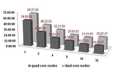
Let's look closer at the scaling factor and the scaling efficiency for this particular job. When requesting 8 cores, the run time will drop to 36% of the time requested for 1 core (on quad core machines). The actual scaling is 2.79 whereas the ideal scaling would be 8. Thus, the efficiency of scaling is only 34.9%. (Scaling efficiency is defined as actual scaling factor / ideal scaling factor. The ideal case is linear scaling and 100% efficiency.) Thus, if you are planning to submit multiple jobs (as part of an LS-OPT study, for example) always request a low number of cores. Each individual job will take longer to run, but the combined run time will be less than if you run on a greater number of cores.
Decomposition efficiency
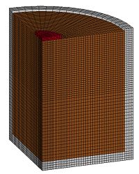
Decomposition is often ignored by LS-DYNA users. However, it allows for a huge savings of computational time for many simulations. Let’s take a look at the problem of soil penetration, with a quarter of the model shown below. In the simulation a rigid pad is pressed down into the soil with the rate of 1 in/sec. The first two inches of penetration are simulated. The Z-axis is pointing upward and the (0,0,0) point is at the top layer of the soil (brown in the figure).
Now consider three different decomposition methods for eight cores, as defined in the pfile:
decomposition 1 - default
decomposition {
   numproc 8
   show
}
decomposition 2 - wedge type
decomposition {
   numproc 8
   C2R 0 0 0 0 0 1 1 0 0
   SY 5000
}
decomposition 3 – cylindrical
decomposition {
   numproc 8
   C2R 0 0 0 0 0 1 1 0 0
   SX 100
}
This gives the three decompositions shown in the figure below:
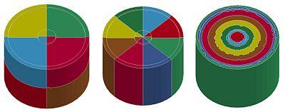
The run time for these jobs is shown in the graph. The third decomposition type was most efficient and allowed for a saving of ~34.7% of the computation time. The second decomposition method gave a saving of ~18.0%.
See Appendix O of the LS-DYNA Keyword User’s Manual, Version 971 for an explanation the use of pfiles.
Also see blog.d3view.com for more interesting information on job decomposition.
Documentation
The LS-DYNA Keyword User’s Manual, Version 971, is on the cluster at /soft/lstc/doc/manuals/ls-dyna_971_manual_k.pdf. Other manuals can be found in the same directory.
LS-PrePost Support has the latest info about LS-PrePost.
LS-DYNA Support also contains a wealth of information about LS-DYNA.
DYNAmore provides technical papers from LS-DYNA conferences also Manuals and FEA Newsletters.
d3VIEW blog tracks developments in LS-DYNA, d3VIEW, and LS-OPT.
LS-DYNA Newsgroup Yahoo LS-DYNA Newsgroup.
LS-PREPOST Newsgroup Questions and answers regarding LS-PREPOST.
Examples and test cases
The 3cars, car2car-ver10, and neon_refined_revised models from TopCrunch are in /soft/lstc/topcrunch.